-
-
Save FloWuenne/b4d1729b5ec2ceecfb4ce532e0fd8d67 to your computer and use it in GitHub Desktop.
| ## Plot PCA for ethnicity of a given VCF file | |
| ## Import publication theme | |
| ## A nice R ggplot theme that I found online. Original can be found here: | |
| ## https://rpubs.com/Koundy/71792 | |
| theme_Publication <- function(base_size=14, base_family="helvetica") { | |
| library(grid) | |
| library(ggthemes) | |
| (theme_foundation(base_size=base_size, base_family=base_family) | |
| + theme(plot.title = element_text(face = "bold", | |
| size = rel(1.2), hjust = 0.5), | |
| text = element_text(), | |
| panel.background = element_rect(colour = NA), | |
| plot.background = element_rect(colour = NA), | |
| panel.border = element_rect(colour = NA), | |
| axis.title = element_text(face = "bold",size = rel(1)), | |
| axis.title.y = element_text(angle=90,vjust =2), | |
| axis.title.x = element_text(vjust = -0.2), | |
| axis.text = element_text(), | |
| axis.line = element_line(colour="black"), | |
| axis.ticks = element_line(), | |
| panel.grid.major = element_line(colour="#f0f0f0"), | |
| panel.grid.minor = element_blank(), | |
| legend.key = element_rect(colour = NA), | |
| legend.position = "bottom", | |
| legend.direction = "horizontal", | |
| legend.key.size= unit(0.2, "cm"), | |
| legend.margin = unit(0, "cm"), | |
| legend.title = element_text(face="italic"), | |
| plot.margin=unit(c(10,5,5,5),"mm"), | |
| strip.background=element_rect(colour="#f0f0f0",fill="#f0f0f0"), | |
| strip.text = element_text(face="bold") | |
| )) | |
| } | |
| scale_fill_Publication <- function(...){ | |
| library(scales) | |
| discrete_scale("fill","Publication",manual_pal(values = c("#386cb0","#fdb462","#7fc97f","#ef3b2c","#662506","#a6cee3","#fb9a99","#984ea3","#ffff33")), ...) | |
| } | |
| scale_colour_Publication <- function(...){ | |
| library(scales) | |
| discrete_scale("colour","Publication",manual_pal(values = c("#386cb0","#fdb462","#7fc97f","#ef3b2c","#662506","#a6cee3","#fb9a99","#984ea3","#ffff33")), ...) | |
| } | |
| ## Import libraries | |
| library(gdsfmt) | |
| library(SNPRelate) | |
| library(ggplot2) | |
| library(ggdendro) | |
| library(RColorBrewer) | |
| library(plyr) | |
| library(dplyr) | |
| ## Set working directory | |
| ## Set color palette for populations | |
| color_palette <- c("#912CEE","#f40000","#4DBD33","#4885ed","#ffc300","#2b2b28") | |
| ## Specify your VCF file | |
| vcf.fn <- "my.vcf" | |
| # Transform the VCF file into gds format | |
| snpgdsVCF2GDS(vcf.fn, "Variants_1000G_exomes.gds", method="biallelic.only") | |
| ## Data Analysis | |
| ## open the newly created gds file | |
| genofile <- snpgdsOpen('Variants_1000G_exomes.gds') | |
| ## LD based SNP pruning | |
| set.seed(1000) | |
| snpset <- snpgdsLDpruning(genofile, ld.threshold=0.2) | |
| snpset.id <- unlist(snpset) | |
| ## Perform PCA on the SNP data | |
| pca <- snpgdsPCA(genofile, snp.id=snpset.id, num.thread=4) | |
| pc.percent <- pca$varprop*100 | |
| head(round(pc.percent, 2)) | |
| ### Plotting | |
| ### Plot results from PCA analysis of variant data | |
| tab12 <- data.frame(sample.id = pca$sample.id, | |
| EV1 = pca$eigenvect[,1], # the first eigenvector | |
| EV2 = pca$eigenvect[,2], # the second eigenvector | |
| stringsAsFactors = FALSE) | |
| tab34 <- data.frame(sample.id = pca$sample.id, | |
| EV3 = pca$eigenvect[,3], # the first eigenvector | |
| EV4 = pca$eigenvect[,4], # the second eigenvector | |
| stringsAsFactors = FALSE) | |
| plot(tab34$EV2, tab34$EV1, xlab="eigenvector 3", ylab="eigenvector 4") | |
| ## Assign ethnicity description from 1000G file | |
| sample.id <- read.gdsn(index.gdsn(genofile, "sample.id")) | |
| populations <- read.table("All_samples_populations.tab",header=T) | |
| tab <- data.frame(sample.id = pca$sample.id, | |
| EV1 = pca$eigenvect[,1], # the first eigenvector | |
| EV2 = pca$eigenvect[,2], # the second eigenvector | |
| stringsAsFactors = FALSE) | |
| colnames(tab) <- c("sample.id","EV1","EV2") | |
| PCA_allVariants2 <- ggplot(tab,aes(x=EV1,y=EV2)) + | |
| geom_point(size=2) + | |
| scale_x_continuous("PC1") + | |
| scale_y_continuous("PC2") + | |
| scale_colour_manual(values=color_palette[1:length(unique(tab$pop))]) + | |
| theme_Publication() | |
| PCA_allVariants2 | |
| ggsave(file="Variants_PCA_pointsize2.svg",plot=PCA_allVariants2) | |
| ggsave(file="Variants_PCA_pointsize1.svg",plot=PCA_allVariants1) |
Hi @krishnakatyal,
In this gist, I specifically combined my data with the snp data from the 1000G to check the ancestry of my samples relative to the 1000G where the ethnicity of participants is known.
This gist is really old and I haven't used this code in a while. I recommend checking out this tutorial, which is very detailed and well written on how to perform PCA analysis on 1000G phase3 data.
https://www.biostars.org/p/335605/
If you just want to plot a PCA plot of your samples, you can use plink. You can convert your vcf file into plink format and then run:
plink --bfile Merge --pca
as explained in step10 of the tutorial I linked!
Hope this helps, let me know if you have any problems/questions!
Thanks alot i was badly struck and your help means alot to me
thanks again!!!!
i will check out the above stuff and will let you know if i have any problems/questions
Again thanks alot
keep safe !!!!
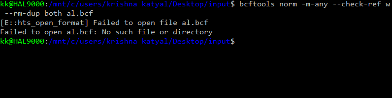
Hello i am getting this error
can you suggest me how to make it right
I apologies for bothering you.

Hey there,
could you please provide some more details for this so I can help you better? Could you provide a reproducible example and post the code and explain which references, files you are using?
I see you are trying to use bcftools to normalize and annotate variants. The error message indicates that there are some variants on the mitochondrial chromosome but that this chromosome is either missing from your reference or annotated differently. I would check how the chromosomes in your file and the reference are annotated. They can either be annotated as 1,2,3,4 or chr1,chr2,chr3,chr4. Usually they have to be annotated the same way in your VCF file and the reference file!
Hello Florian
I removed the chrM from my data file then change the chr1 chr2 chr3 into 1 2 3 as per the fasta file to make the vcf file and the fasta file have the same.I am using the GRCh37 / hg19 reference genome.
first i was gettinh chrM not found then i removed the chrM and i get the chr1 not found error which explains the difference between my fasta and my vcf file so i used emeditor an editor to change my vcf file (as other methods were not preserving the header).
now chrM is gone the annotation of fasta and vcf is same but still i get the error
code :
bcftools norm -m-any --check-ref w -f human_g1k_v37.fasta \
data.vcf | \
bcftools annotate -x ID -I +'%CHROM:%POS:%REF:%ALT' | \
bcftools norm -Ob --rm-dup both \
> data.bcf ;
`
I am giving to the orginal data(it is single sample) which will make it is easier for check the annotation error
Link to my data
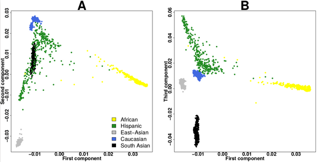
I think the plot should look like this(like the plot in the biostar tutorial)
Thanks alot for helping and keef safe !
i wish for your best health
I want to do pca of a data and the data is in vcf format but i dont have the 'Variants_1000G_exomes.gds' file can you please give me advice what to do...i am new in this field.
thanks!!!